Response by Marcott et al.
Readers will be aware of the paper by Shaun Marcott and colleagues, that they published a couple weeks ago in the journal Science. That paper sought to extend the global temperature record back over the entire Holocene period, i.e. just over 11 kyr back time, something that had not really been attempted before. The paper got a fair amount of media coverage (see e.g. this article by Justin Gillis in the New York Times). Since then, a number of accusations from the usual suspects have been leveled against the authors and their study, and most of it is characteristically misleading. We are pleased to provide the authors’ response, below. Our view is that the results of the paper will stand the test of time, particularly regarding the small global temperature variations in the Holocene. If anything, early Holocene warmth might be overestimated in this study.
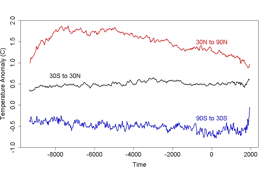
Update: Tamino has three excellent posts in which he shows why the Holocene reconstruction is very unlikely to be affected by possible discrepancies in the most recent (20th century) part of the record. The figure showing Holocene changes by latitude is particularly informative.
____________________________________________
Prepared by Shaun A. Marcott, Jeremy D. Shakun, Peter U. Clark, and Alan C. Mix
Primary results of study
Global Temperature Reconstruction: We combined published proxy temperature records from across the globe to develop regional and global temperature reconstructions spanning the past ~11,300 years with a resolution >300 yr; previous reconstructions of global and hemispheric temperatures primarily spanned the last one to two thousand years. To our knowledge, our work is the first attempt to quantify global temperature for the entire Holocene.
Structure of the Global and Regional Temperature Curves: We find that global temperature was relatively warm from approximately 10,000 to 5,000 years before present. Following this interval, global temperature decreased by approximately 0.7°C, culminating in the coolest temperatures of the Holocene around 200 years before present during what is commonly referred to as the Little Ice Age. The largest cooling occurred in the Northern Hemisphere.
Holocene Temperature Distribution: Based on comparison of the instrumental record of global temperature change with the distribution of Holocene global average temperatures from our paleo-reconstruction, we find that the decade 2000-2009 has probably not exceeded the warmest temperatures of the early Holocene, but is warmer than ~75% of all temperatures during the Holocene. In contrast, the decade 1900-1909 was cooler than~95% of the Holocene. Therefore, we conclude that global temperature has risen from near the coldest to the warmest levels of the Holocene in the past century. Further, we compare the Holocene paleotemperature distribution with published temperature projections for 2100 CE, and find that these projections exceed the range of Holocene global average temperatures under all plausible emissions scenarios.
Frequently Asked Questions and Answers
Q: What is global temperature?A: Global average surface temperature is perhaps the single most representative measure of a planet’s climate since it reflects how much heat is at the planet’s surface. Local temperature changes can differ markedly from the global average. One reason for this is that heat moves around with the winds and ocean currents, warming one region while cooling another, but these regional effects might not cause a significant change in the global average temperature. A second reason is that local feedbacks, such as changes in snow or vegetation cover that affect how a region reflects or absorbs sunlight, can cause large local temperature changes that are not mirrored in the global average. We therefore cannot rely on any single location as being representative of global temperature change. This is why our study includes data from around the world.
We can illustrate this concept with temperature anomaly data based on instrumental records for the past 130 years from the National Climatic Data Center (http://www.ncdc.noaa.gov/cmb-faq/anomalies.php#anomalies). Over this time interval, an increase in the global average temperature is documented by thermometer records, rising sea levels, retreating glaciers, and increasing ocean heat content, among other indicators.
Yet if we plot temperature anomaly data since 1880 at the same locations as the 73 sites used in our paleotemperature study, we see that the data are scattered and the trend is unclear. When these same 73 historical temperature records are averaged together, we see a clear warming signal that is very similar to the global average documented from many more sites (Figure 1). Averaging reduces local noise and provides a clearer perspective on global climate.

New Scientist magazine has an “app” that allows one to point-and-plot instrumental temperatures for any spot on the map to see how local temperature changes compare to the global average over the past century (http://warmingworld.newscientistapps.com/).
Q: How does one go about reconstructing temperatures in the past?
A: Changes in Earth’s temperature for the last ~160 years are determined from instrumental data, such as thermometers on the ground or, for more recent times, satellites looking down from space. Beyond about 160 years ago, we must turn to other methods that indirectly record temperature (called “proxies”) for reconstructing past temperatures. For example, tree rings, calibrated to temperature over the instrumental era, provide one way of determining temperatures in the past, but few trees extend beyond the past few centuries or millennia. To develop a longer record, we used primarily marine and terrestrial fossils, biomolecules, or isotopes that were recovered from ocean and lake sediments and ice cores. All of these proxies have been independently calibrated to provide reliable estimates of temperature.
Q: Did you collect and measure the ocean and land temperature data from all 73 sites?
A: No. All of the datasets were previously generated and published in peer-reviewed scientific literature by other researchers over the past 15 years. Most of these datasets are freely available at several World Data Centers (see links below); those not archived as such were graciously made available to us by the original authors. We assembled all these published data into an easily used format, and in some cases updated the calibration of older data using modern state-of-the-art calibrations. We made all the data available for download free-of-charge from the Science web site (see link below). Our primary contribution was to compile these local temperature records into “stacks” that reflect larger-scale changes in regional and global temperatures. We used methods that carefully consider potential sources of uncertainty in the data, including uncertainty in proxy calibration and in dating of the samples (see step-by-step methods below).
NOAA National Climate Data Center: http://www.ncdc.noaa.gov/paleo/paleo.html
PANGAEA: http://www.pangaea.de/
Holocene Datasets: http://www.sciencemag.org/content/339/6124/1198/suppl/DC1
Q: Why use marine and terrestrial archives to reconstruct global temperature when we have the ice cores from Greenland and Antarctica?
A: While we do use these ice cores in our study, they are limited to the polar regions and so give only a local or regional picture of temperature changes. Just as it would not be reasonable to use the recent instrumental temperature history from Greenland (for example) as being representative of the planet as a whole, one would similarly not use just a few ice cores from polar locations to reconstruct past temperature change for the entire planet.
Q: Why only look at temperatures over the last 11,300 years?
A: Our work was the second half of a two-part study assessing global temperature variations since the peak of the last Ice Age about 22,000 years ago. The first part reconstructed global temperature over the last deglaciation (22,000 to 11,300 years ago) (Shakun et al., 2012, Nature 484, 49-55; see also http://www.people.fas.harvard.edu/~shakun/FAQs.html), while our study focused on the current interglacial warm period (last 11,300 years), which is roughly the time span of developed human civilizations.
Q: Is your paleotemperature reconstruction consistent with reconstructions based on the tree-ring data and other archives of the past 2,000 years?
A: Yes, in the parts where our reconstruction contains sufficient data to be robust, and acknowledging its inherent smoothing. For example, our global temperature reconstruction from ~1500 to 100 years ago is indistinguishable (within its statistical uncertainty) from the Mann et al. (2008) reconstruction, which included many tree-ring based data. Both reconstructions document a cooling trend from a relatively warm interval (~1500 to 1000 years ago) to a cold interval (~500 to 100 years ago, approximately equivalent to the Little Ice Age).
Q: What do paleotemperature reconstructions show about the temperature of the last 100 years?
A: Our global paleotemperature reconstruction includes a so-called “uptick” in temperatures during the 20th-century. However, in the paper we make the point that this particular feature is of shorter duration than the inherent smoothing in our statistical averaging procedure, and that it is based on only a few available paleo-reconstructions of the type we used. Thus, the 20th century portion of our paleotemperature stack is not statistically robust, cannot be considered representative of global temperature changes, and therefore is not the basis of any of our conclusions. Our primary conclusions are based on a comparison of the longer term paleotemperature changes from our reconstruction with the well-documented temperature changes that have occurred over the last century, as documented by the instrumental record. Although not part of our study, high-resolution paleoclimate data from the past ~130 years have been compiled from various geological archives, and confirm the general features of warming trend over this time interval (Anderson, D.M. et al., 2013, Geophysical Research Letters, v. 40, p. 189-193; http://www.agu.org/journals/pip/gl/2012GL054271-pip.pdf).
Q: Is the rate of global temperature rise over the last 100 years faster than at any time during the past 11,300 years?
A: Our study did not directly address this question because the paleotemperature records used in our study have a temporal resolution of ~120 years on average, which precludes us from examining variations in rates of change occurring within a century. Other factors also contribute to smoothing the proxy temperature signals contained in many of the records we used, such as organisms burrowing through deep-sea mud, and chronological uncertainties in the proxy records that tend to smooth the signals when compositing them into a globally averaged reconstruction.
We showed that no temperature variability is preserved in our reconstruction at cycles shorter than 300 years, 50% is preserved at 1000-year time scales, and nearly all is preserved at 2000-year periods and longer. Our Monte-Carlo analysis accounts for these sources of uncertainty to yield a robust (albeit smoothed) global record. Any small “upticks” or “downticks” in temperature that last less than several hundred years in our compilation of paleoclimate data are probably not robust, as stated in the paper.
Q: How do you compare the Holocene temperatures to the modern instrumental data?
A: One of our primary conclusions is based on Figure 3 of the paper, which compares the magnitude of global warming seen in the instrumental temperature record of the past century to the full range of temperature variability over the entire Holocene based on our reconstruction. We conclude that the average temperature for 1900-1909 CE in the instrumental record was cooler than ~95% of the Holocene range of global temperatures, while the average temperature for 2000-2009 CE in the instrumental record was warmer than ~75% of the Holocene distribution. As described in the paper and its supplementary material, Figure 3 provides a reasonable assessment of the full range of Holocene global average temperatures, including an accounting for high-frequency changes that might have been damped out by the averaging procedure.
Q: What about temperature projections for the future?
A: Our study used projections of future temperature published in the Fourth Assessment of the Intergovernmental Panel on Climate Change in 2007, which suggest that global temperature is likely to rise 1.1-6.4°C by the end of the century (relative to the late 20th century), depending on the magnitude of anthropogenic greenhouse gas emissions and the sensitivity of the climate to those emissions.
Figure 3 in the paper compares these published projected temperatures from various emission scenarios to our assessment of the full distribution of Holocene temperature distributions. For example, a middle-of-the-road emission scenario (SRES A1B) projects global mean temperatures that will be well above the Holocene average by the year 2100 CE. Indeed, if any of the six emission scenarios considered by the IPCC that are shown on Figure 3 are followed, future global average temperatures, as projected by modeling studies, will likely be well outside anything the Earth has experienced in the last 11,300 years, as shown in Figure 3 of our study.

Technical Questions and Answers:
Q. Why did you revise the age models of many of the published records that were used in your study?
A. The majority of the published records used in our study (93%) based their ages on radiocarbon dates. Radiocarbon is a naturally occurring isotope that is produced mainly in the upper atmosphere by cosmic rays. This form of carbon is then distributed around the world and incorporated into living things. Dating is based on the amount of this carbon left after radioactive decay. It has been known for several decades that radiocarbon years differ from true “calendar” years because the amount of radiocarbon produced in the atmosphere changes over time, as does the rate that carbon is exchanged between the ocean, atmosphere, and biosphere. This yields a bias in radiocarbon dates that must be corrected. Scientists have been able to determine the correction between radiocarbon years and true calendar year by dating samples of known age (such as tree samples dated by counting annual rings) and comparing the apparent radiocarbon age to the true age.
Through many careful measurements of this sort, they have demonstrated that, in general, radiocarbon years become progressively “younger” than calendar years as one goes back through time. For example, the ring of a tree known to have grown 5700 years ago will have a radiocarbon age of ~5000 years, whereas one known to have grown 12,800 years ago will have a radiocarbon age of ~11,000 years.
For our paleotemperature study, all radiocarbon ages needed to be converted (or calibrated) to calendar ages in a consistent manner. Calibration methods have been improved and refined over the past few decades. Because our compilation included data published many years ago, some of the original publications used radiocarbon calibration systems that are now obsolete. To provide a consistent chronology based on the best current information, we thus recalibrated all published radiocarbon ages with Calib 6.0.1 software (using the databases INTCAL09 for land samples or MARINE09 for ocean samples) and its state-of-the-art protocol for site-specific locations and materials. This software is freely available for online use at http://calib.qub.ac.uk/calib/.
By convention, radiocarbon dates are recorded as years before present (BP). BP is universally defined as years before 1950 CE, because after that time the Earth’s atmosphere became contaminated with artificial radiocarbon produced as a bi-product of nuclear bomb tests. As a result, radiocarbon dates on intervals younger than 1950 are not useful for providing chronologic control in our study.
After recalibrating all radiocarbon control points to make them internally consistent and in compliance with the scientific state-of-the-art understanding, we constructed age models for each sediment core based on the depth of each of the calibrated radiocarbon ages, assuming linear interpolation between dated levels in the core, and statistical analysis that quantifies the uncertainty of ages between the dated levels.
In geologic studies it is quite common that the youngest surface of a sediment core is not dated by radiocarbon, either because the top is disturbed by living organisms or during the coring process. Moreover, within the past hundred years before 1950 CE, radiocarbon dates are not very precise chronometers, because changes in radiocarbon production rate have by coincidence roughly compensated for fixed decay rates. For these reasons, and unless otherwise indicated, we followed the common practice of assuming an age of 0 BP for the marine core tops.
Q: Are the proxy records seasonally biased?
A: Maybe. We cannot exclude the possibility that some of the paleotemperature records are biased toward a particular season rather than recording true annual mean temperatures. For instance, high-latitude proxies based on short-lived plants or other organisms may record the temperature during the warmer and sunnier summer months when the organisms grow most rapidly. As stated in the paper, such an effect could impact our paleo-reconstruction. For example, the long-term cooling in our global paleotemperature reconstruction comes primarily from Northern Hemisphere high-latitude marine records, whereas tropical and Southern Hemisphere trends were considerably smaller.
This northern cooling in the paleotemperature data may be a response to a long-term decline in summer insolation associated with variations in the earth’s orbit, and this implies that the paleotemperature proxies here may be biased to the summer season. A summer cooling trend through Holocene time, if driven by orbitally modulated seasonal insolation, might be partially canceled out by winter warming due to well-known orbitally driven rise in Northern-Hemisphere winter insolation through Holocene time. Summer-biased proxies would not record this averaging of the seasons. It is not currently possible to quantify this seasonal effect in the reconstructions.
Qualitatively, however, we expect that an unbiased recorder of the annual average would show that the northern latitudes might not have cooled as much as seen in our reconstruction. This implies that the range of Holocene annual-average temperatures might have been smaller in the Northern Hemisphere than the proxy data suggest, making the observed historical temperature averages for 2000-2009 CE, obtained from instrumental records, even more unusual with respect to the full distribution of Holocene global-average temperatures.
Q: What do paleotemperature reconstructions show about the temperature of the last 100 years?
A: Here we elaborate on our short answer to this question above. We concluded in the published paper that “Without filling data gaps, our Standard5×5 reconstruction (Figure 1A) exhibits 0.6°C greater warming over the past ~60 yr B.P. (1890 to 1950 CE) than our equivalent infilled 5° × 5° area-weighted mean stack (Figure 1, C and D). However, considering the temporal resolution of our data set and the small number of records that cover this interval (Figure 1G), this difference is probably not robust.”
This statement follows from multiple lines of evidence that are presented in the paper and the supplementary information: (1) the different methods that we tested for generating a reconstruction produce different results in this youngest interval, whereas before this interval, the different methods of calculating the stacks are nearly identical (Figure 1D), (2) the median resolution of the datasets (120 years) is too low to statistically resolve such an event, (3) the smoothing presented in the online supplement results in variations shorter than 300 yrs not being interpretable, and (4) the small number of datasets that extend into the 20th century (Figure 1G) is insufficient to reconstruct a statistically robust global signal, showing that there is a considerable reduction in the correlation of Monte Carlo reconstructions with a known (synthetic) input global signal when the number of data series in the reconstruction is this small (Figure S13).
Q: How did you create the Holocene paleotemperature stacks?
A: We followed these steps in creating the Holocene paleotemperature stacks:
1. Compiled 73 medium-to-high resolution calibrated proxy temperature records spanning much or all of the Holocene.
2. Calibrated all radiocarbon ages for consistency using the latest and most precise calibration software (Calib 6.0.1 using INTCAL09 (terrestrial) or MARINE09 (oceanic) and its protocol for the site-specific locations and materials) so that all radiocarbon-based records had a consistent chronology based on the best current information. This procedure updates previously published chronologies, which were based on a variety of now-obsolete and inconsistent calibration methods.
3. Where applicable, recalibrated paleotemperature proxy data based on alkenones and TEX86using consistent calibration equations specific to each of the proxy types.
4. Used a Monte Carlo analysis to generate 1000 realizations of each proxy record, linearly interpolated to constant time spacing, perturbing them with analytical uncertainties in the age model and temperature estimates, including inflation of age uncertainties between dated intervals. This procedure results in an unbiased assessment of the impact of such uncertainties on the final composite.
5. Referenced each proxy record realization as an anomaly relative to its mean value between 4500 and 5500 years Before Present (the common interval of overlap among all records; Before Present, or BP, is defined by standard practice as time before 1950 CE).
6. Averaged the first realization of each of the 73 records, and then the second realization of each, then the third, the fourth, and so on, to form 1000 realizations of the global or regional temperature stacks.
7. Derived the mean temperature and standard deviation from the 1000 simulations of the global temperature stack.
8. Repeated this procedure using several different area-weighting schemes and data subsets to test the sensitivity of the reconstruction to potential spatial and proxy biases in the dataset.
9. Mean-shifted the global temperature reconstructions to have the same average as the Mann et al. (2008) CRU-EIV temperature reconstruction over the interval 510-1450 years Before Present. Since the CRU-EIV reconstruction is referenced as temperature anomalies from the 1961-1990 CE instrumental mean global temperature, the Holocene reconstructions are now also effectively referenced as anomalies from the 1961-1990 CE mean.
10. Estimated how much higher frequency (decade-to-century scale) variability is plausibly missing from the Holocene reconstruction by calculating attenuation as a function of frequency in synthetic data processed with the Monte-Carlo stacking procedure, and by statistically comparing the amount of temperature variance the global stack contains as a function of frequency to the amount contained in the CRU-EIV reconstruction. Added this missing variability to the Holocene reconstruction as red noise.
11. Pooled all of the Holocene global temperature anomalies into a single histogram, showing the distribution of global temperature anomalies during the Holocene, including the decadal-to century scale high-frequency variability that the Monte-Carlo procedure may have smoothed from the record (largely from the accounting for chronologic uncertainties).
12. Compared the histogram of Holocene paleotemperatures to the instrumental global temperature anomalies during the decades 1900-1909 CE and 2000-2009 CE. Determined the fraction of the Holocene temperature anomalies colder than 1900-1909 CE and 2000-2009 CE.
13. Compared global temperature projections for 2100 CE from the Fourth Assessment Report of the Intergovernmental Panel on Climate Change for various emission scenarios.
14. Evaluated the impact of potential sources of uncertainty and smoothing in the Monte-Carlo procedure, as a guide for future experimental design to refine such analyses.
Copied from:
No comments:
Post a Comment